Custom Split Example#

Import core libraries:

from pathlib import Path
import plinder 

from plinder.data.splits import (
    split,
    get_default_config,
)
from plinder.core.scores import query_index

plinder_cfg = plinder.core.get_config()
plinder_local_storage = plinder_cfg.data.plinder_dir

Split Config#

First, let’s modify the split config. We will first get the default config using get_default_config() and then change some of the parameters.

cfg = get_default_config() 
print(f'Validation set size: {cfg.split.num_val}')
print(f'Test set size: {cfg.split.num_test}')
print(f'Minimum size of each cluster in the validation set: {cfg.split.min_val_cluster_size}')

Validation set size: 1000
Test set size: 1000
Minimum size of each cluster in the validation set: 30

Since we reduced the total number of samples, let’s also reduce the minimum validation set cluster size, so we avoid removing to many systems.
All configs can be found here

cfg.split.num_test = 500 # Reduce the max size of the test set
cfg.split.num_val = 500 # Reduce the max size of the validation set
cfg.split.min_val_cluster_size = 5 # Reduce the minimum required size of each cluster in the validation set

Custom Dataset#

Let’s generate a custom dataset that we want to resplit. First, let’s load the plindex and then create a custom dataset.

cols_of_interest = [
    "system_id",
    "entry_pdb_id",
    "ligand_ccd_code",
    "ligand_binding_affinity",
    "ligand_is_proper",
    "ligand_molecular_weight",
    "system_has_binding_affinity",
]
custom_df = query_index(
    columns=cols_of_interest, splits=["train", "val", "test", "removed"] 
)

2024-10-25 11:14:50,015 | plinder.core.utils.cpl.download_paths:24 | INFO : runtime succeeded: 0.53s
2024-10-25 11:14:51,601 | plinder.core.utils.cpl.download_paths:24 | INFO : runtime succeeded: 0.55s

custom_df.shape

(567394, 8)

Let’s filter every system out that doesn’t have a binding affinity system_has_binding_affinity, ions and artifacts ligand_is_proper and ligands with a molecular weight of less than 400 g/mol ligand_molecular_weight.

custom_df = custom_df[
    (custom_df["ligand_is_proper"] == True) &
    (custom_df["system_has_binding_affinity"] == True) &
    (custom_df["ligand_molecular_weight"] > 400)
]
custom_df.head(4)

	system_id	entry_pdb_id	ligand_ccd_code	ligand_binding_affinity	ligand_is_proper	ligand_molecular_weight	system_has_binding_affinity	split
20	2grt__1__1.A_2.A__1.C	2grt	GDS	6.079633	True	612.151962	True	train
22	2grt__1__1.A_2.A__2.C	2grt	GDS	6.079633	True	612.151962	True	train
74	8gr9__1__1.A_1.B__1.C_1.J	8gr9	COA	5.465907	True	767.115209	True	removed
85	1grn__1__1.A_1.B__1.C_1.D_1.E	1grn	GDP	3.428291	True	443.024330	True	train

custom_df.shape

(36247, 8)

custom_df['split'].value_counts()

split
train      25610
removed    10483
val           92
test          62
Name: count, dtype: int64

Resplitting the Dataset#

We see that we end up with only 92 systems in our validation set and 62 in our test set. We also have over 10k removed systems. Let’s resplit the dataset and see how the new split looks like.

NOTE: resplitting the dataset requires a lot of memory and might only be feasible on a HPC cluster.

data_dir = Path(plinder_local_storage)
custom_systems = set(custom_df['system_id'].unique())
split_name = 'custom_1'

new_split_df = split(
    data_dir=data_dir,
    cfg=cfg, # here we use the modified config from earlier
    relpath=split_name,
    selected_systems=custom_systems 
)
new_split_df.shape

(33047, 13)

new_split_df.head(4)

	system_id	uniqueness	split	cluster	cluster_for_val_split	system_pass_validation_criteria	system_pass_statistics_criteria	system_proper_num_ligand_chains	system_proper_num_pocket_residues	system_proper_num_interactions	system_proper_ligand_max_molecular_weight	system_has_binding_affinity	system_has_apo_or_pred
0	10gs__1__1.A_1.B__1.C	10gs__A_B__C_c101993	train	c62	c0	True	True	1	24	15	473.162057	True	False
1	10gs__1__1.A_1.B__1.E	10gs__A_B__E_c101949	train	c62	c0	True	True	1	24	13	473.162057	True	False
2	19gs__1__1.A_1.B__1.C_1.D	19gs__A_B__C_D_c147080	train	c62	c0	False	True	2	30	12	787.630334	True	False
3	19gs__1__1.A_1.B__1.F_1.G	19gs__A_B__F_G_c101954	train	c62	c0	False	True	2	30	14	787.630334	True	False

Visualizing the new Split#

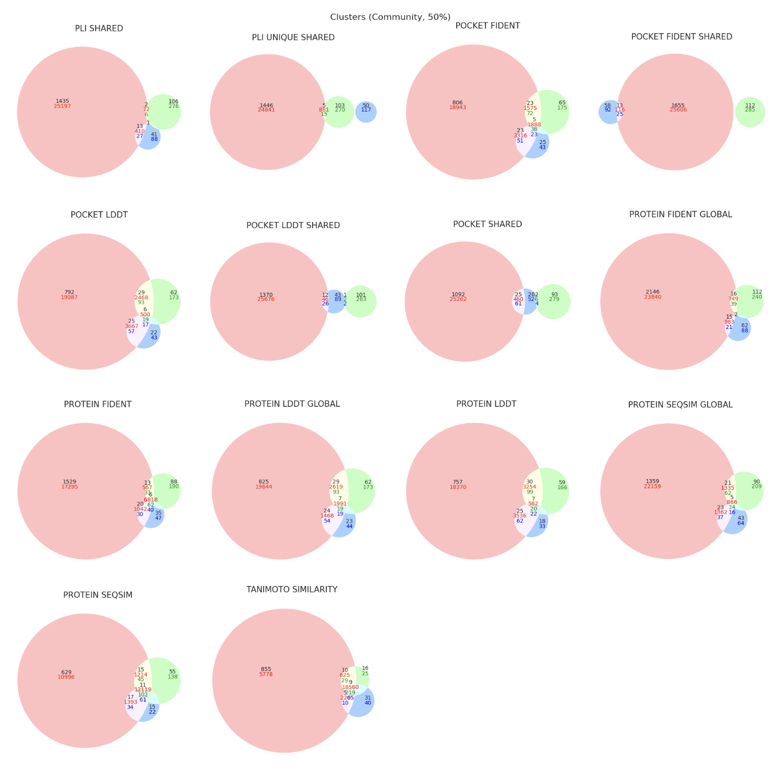
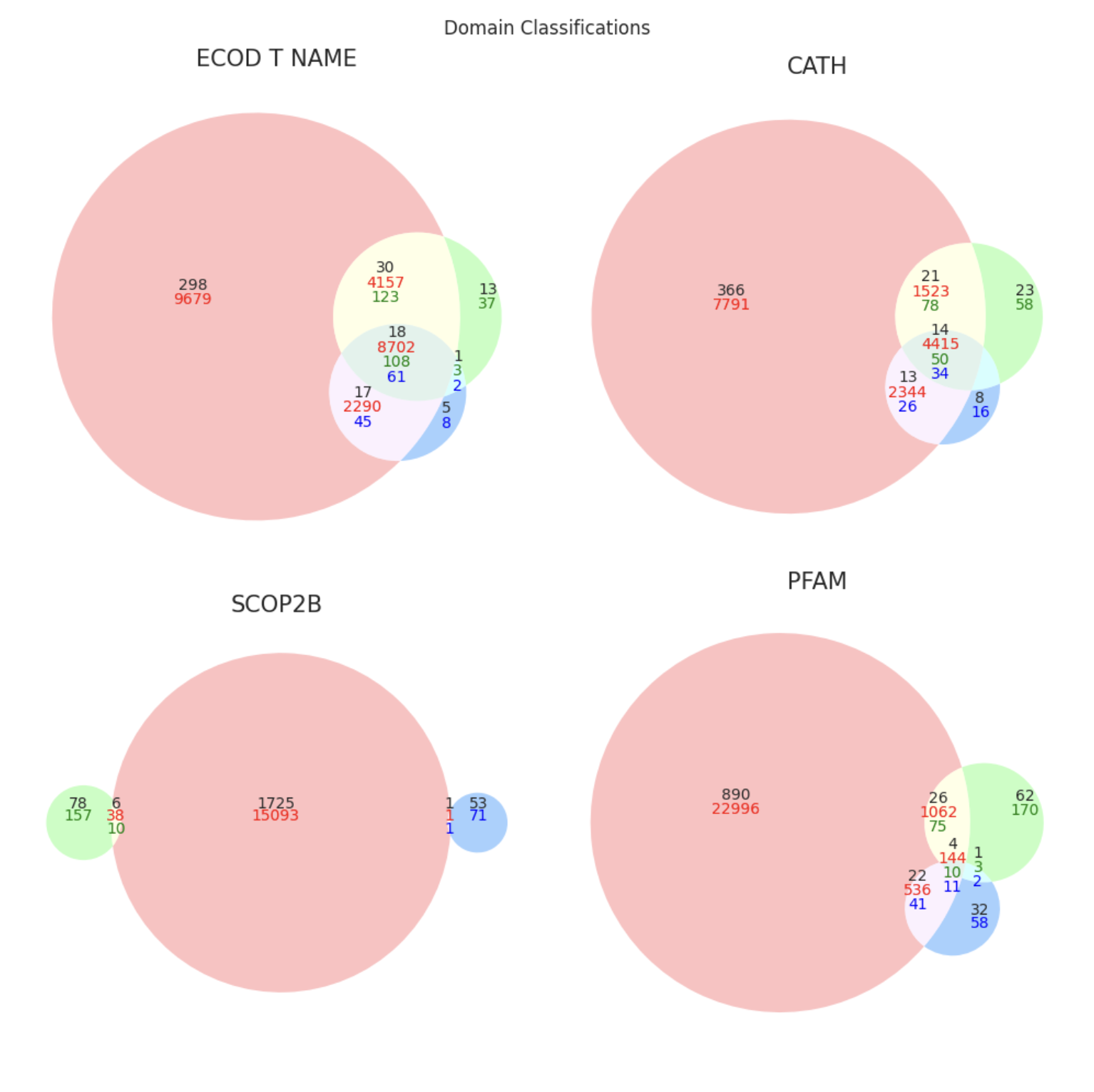
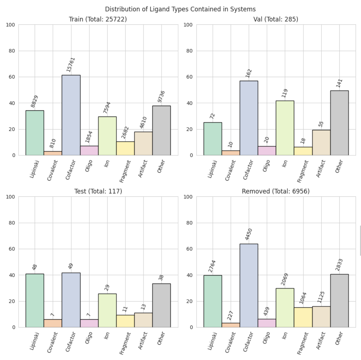
Now that we have our first custom split, let’s use the SplitPropertiesPlotter to visualize the new split.

from plinder.core.split.plot import SplitPropertiesPlotter

plotter = SplitPropertiesPlotter.from_files(
    data_dir = Path(plinder_local_storage),
    split_file = Path(f'{plinder_local_storage}/splits/split_{split_name}.parquet'),
)

This will create a folder split_plots in the current working directory with the following plots:

split_plots/split_proportions.png

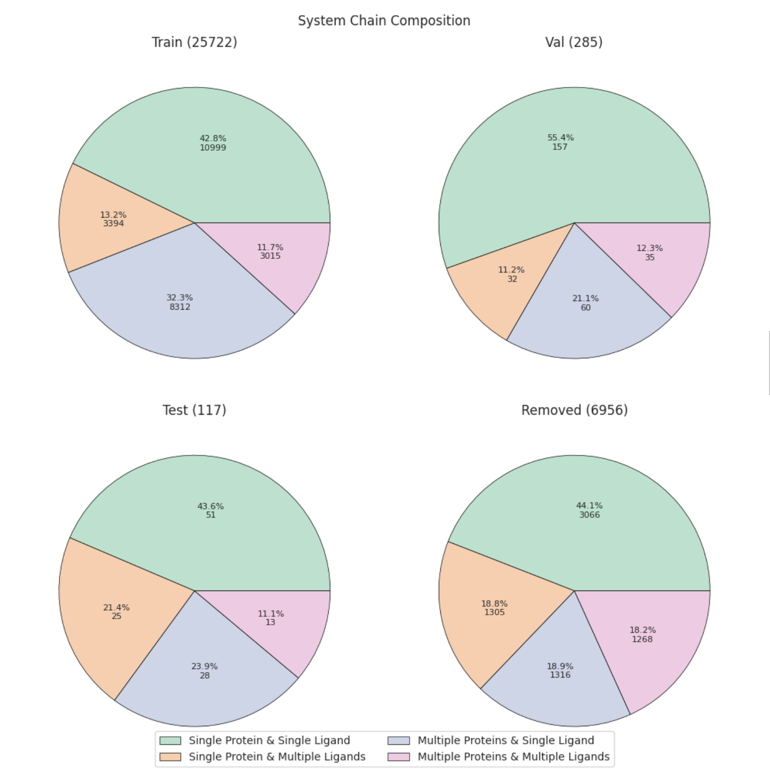
split_plots/chain_composition.png

split_plots/domain_classifications.png

split_plots/ligand_types.png

split_plots/molecular_descriptors.png

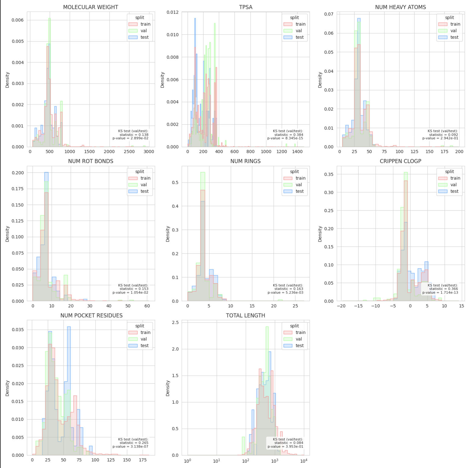
split_plots/priorities.png

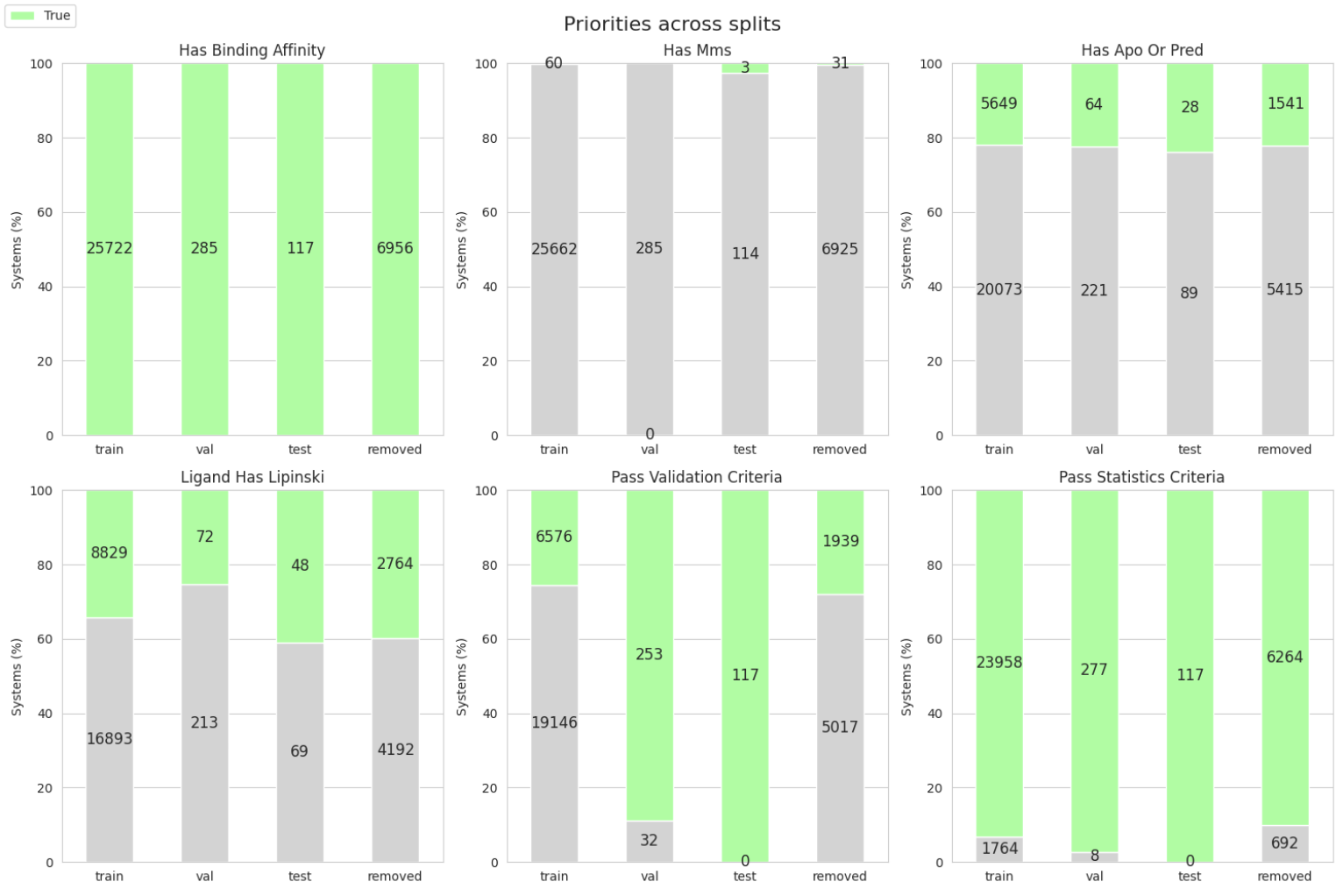
split_plots/plinder_clusters.png